How To Get Negative Percentages In Parentheses In Excel
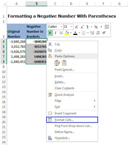
Select the cells right click on the mouse. Or by clicking on this icon in the ribbon Code to customize numbers in Excel.

7 Amazing Excel Custom Number Format Tricks You Must Know
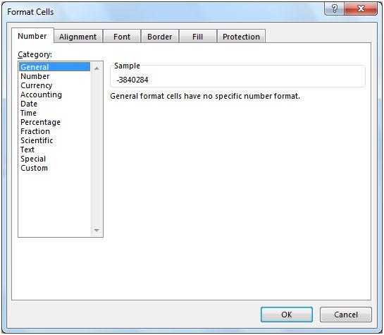
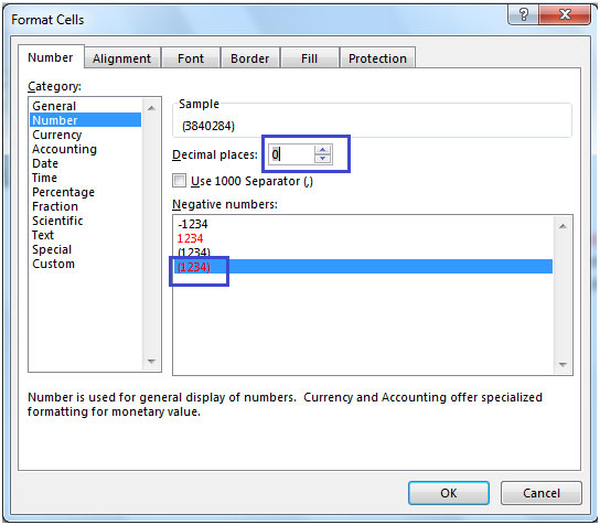
On the Numbers tab for Negative number format choose 11 On the Currency tab for Negative currency format choose 11 Click OK and then click OK again.

How to get negative percentages in parentheses in excel. Select the modeling tab. Now select the cells to which to apply this formatting. If you want to calculate a percentage of a number in excel simply multiply the percentage value by the number that you want the percentage ofTake the above data for example you can quickly find the percentage of a specific option with following formulaThe formula in parentheses calculates the percentage which the remainder of the formula.
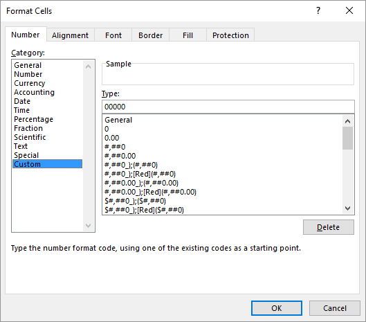
In the Format Cells box in the Category list click Custom. Negative Percentage in Parenthesis instead of with - sign. Click on the Home tab on the top of the window and click Format button in the cells section and select format cells option.
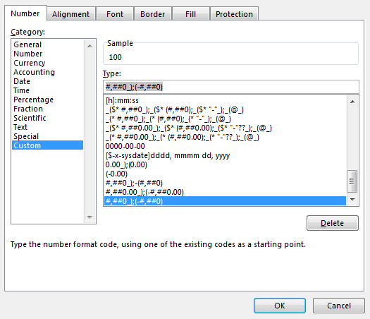
Enter the custom format above. I need to display with the parenthesis 136for negative. Open your file in Excel.
000 hope this will work for you. You can also change the font color to red. How about a custom format of.
Enter 0 in the Decimal places box to avoid decimals. Follow these steps to display parentheses around negative numbers. In the Type box enter the following format.
The only difference between mathematical excel percentage calculation is in excel 100 is missing because in excel when calculating a percent you dont have to multiply the resulting lets check out various available options or formulas on how to calculate a percentage increase in excel. Hi Right click on the cell you want to format choos format cells choos the. You can learn more about these regional settings on Microsofts website.
There is a more in depth article here about custom number formats. To select multiple cells hold down the Ctrl key as you. Click on Format Cells.
Open the dialog box Format Cells using the shortcut Ctrl 1 or by clicking on the last option of the Number Format dropdown list. Click on Format Cells orPress Ctrl1 on the keyboard to open the Format Cells dialog box. Number tab choos custom enter in the Type text box.
In this case I choose the red color and bold font for the negative percentage. Select the cell or cells that contain negative percentages. You can always use a custom format FormatCellsNumberCustom Type.
In the Negative Numbers box select the 3rd option as highlighted. Add Brackets. Use your mouse to select the cells of the spreadsheet.
Now it returns to the New Formatting Rule dialog box please click the OK button to finish the rule creating. On the Home tab click Format Format Cells. Then the numbers line up.
Select the Number tab and from Category select Number. For example you may want to show an expense of 5000 as 5000 or -5000. Right click on the cell that you want to format.
To display your negative numbers with parentheses we must create our own number format. Add Parenthesis to Negative Percentages. Use the custom format.
Then click the OK button. To so so follow the following steps. When a formula returns a negative percentage the result is formatted as -49.
From the Number sub menu select Custom. Is the order of that formatting string. I have been able to format single cells to display negative percents Budget to Actual hours but I cannot copy the formatting to cells with positive percents without eliminating the format style I want.
In accounting and financial models sometimes you will want to show negative numbers in brackets and in red color. The _ and _ just reserve room for the and. In the Format Cells dialog box specify your desire format.
How to display negative numbers in brackets in excel. Change it to a decimal format then Custom. You can do this on the Modeling tab of the desktop.
If you want a minus sign in front of your negative financial values rather than enclosing them in parentheses select the Currency format on the Number Format drop-down menu or on the Number tab of the Format Cells dialog box. In this Advanced Excel tutorial you are going to learn ways. When a formula returns a negative percentage.
In parentheses you can choose red or black In the UK and many other European countries youll typically be able to set negative numbers to show in black or red and with or without a minus sign in both colors but have no option for parentheses. Is there any format in Excel 2002 that allows for it to be formatted 49. Add Brackets Minus Sign Mark Red All Negative PercentagesIn this Excel tutorial you ar.

Displaying Negative Numbers In Parentheses Excel

Pin By Lwhite1413 On Knowledge Excel Shortcuts Microsoft Excel Tutorial Excel Tutorials
Displaying Negative Percentages In Red Microsoft Excel

Pin By B Collection On Quotes Physics Memes Negative Numbers How To Apply
How To Display Negative Numbers In Brackets In Excel Free Excel Tutorial

Displaying Negative Numbers In Parentheses Excel

Displaying Negative Numbers In Parentheses Excel

Displaying Negative Numbers In Parentheses Excel

Excel Negative Numbers In Brackets Auditexcel Co Za
Formatting A Negative Number With Parentheses In Microsoft Excel

How To Display Negative Percentages In Red Within Brackets In Excel Excel Tutorials Excel Negativity

Excel Negative Numbers In Red Or Another Colour Auditexcel Co Za
Formatting A Negative Number With Parentheses In Microsoft Excel

How To Write Copyright Sign C In Microsoft Excel Microsoft Excel Excel Tutorials Excel

How To Shrink Text To Fit Inside A Cell In Excel Without Vba Excel Tutorials Excel Cell

Pin By Thinking Value On Computer Elementary School Computer Lab Excel Tutorials Technology Lessons
Formatting A Negative Number With Parentheses In Microsoft Excel
Formatting A Negative Number With Parentheses In Microsoft Excel
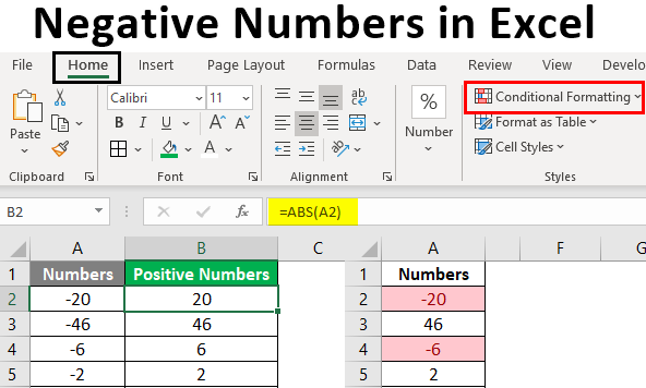
Negative Numbers In Excel How To Use Negative Numbers In Excel